
Pushover Analysis in ETABS: Automatic Determination of the Target Displacement According to Eurocode 8
Nonlinear static analysis, or pushover analysis, has become a central tool in the seismic assessment of existing buildings. Instead of reducing nonlinear response to a behavior factor, the structure is pushed laterally in incremental steps and its transition into the plastic range is observed, including plastic hinge formation and its actual deformation capacity. The key question is therefore simple: what displacement will the design earthquake effectively impose on the structure? That value is the target displacement.
This article shows how ETABS automatically determines the target displacement following the N2 method prescribed in Annex B of EN 1998-1. The objective is not merely to run a command: it is to examine in detail what the software does, so that each reported value can be checked manually and linked to the corresponding code clause.
The case study is a typical 1960s reinforced-concrete building located in Lisbon, with eight stories, a mixed frame-wall structural system, and ribbed slabs, assessed for the Significant Damage (SD) limit state according to EC8-3.
From the Capacity Curve to the Target Displacement
The primary result of a pushover analysis is the capacity curve: the base shear Fb as a function of the displacement of a control node dn, usually the center of mass of the roof. This curve summarizes, in a single plot, the initial stiffness, progressive yielding, and degradation of the structure.
In the model analyzed here, the pushover analyses are nonlinear cases that start from the loaded state under gravity loads (G+ψ₂Q), use displacement control at the roof control node, and include second-order effects (P-Delta). For each direction, two vertical distributions of lateral forces are defined: uniform, proportional to mass, and modal, proportional to the fundamental mode, as summarized in the following table.
| Load case | Distribution | Direction | Pattern | SF | 2nd order |
|---|---|---|---|---|---|
| push_modal_X | Modal | X (U1) | Mode 1 | +1 | P-Delta |
| push_modal_Y+ | Modal | Y (U2) | Mode 3 | +1 | P-Delta |
| push_modal_Y− | Modal | Y (U2) | Mode 3 | −1 | P-Delta |
| push_unif_X | Uniform | X (U1) | UX acceleration | −1 | P-Delta |
| push_unif_Y+ | Uniform | Y (U2) | UY acceleration | −1 | P-Delta |
| push_unif_Y− | Uniform | Y (U2) | UY acceleration | +1 | P-Delta |
All cases use the Event-to-Event solution scheme and save multiple states (50 to 100) to represent the curve. The control node is common to all cases, and the initial monitored displacement is set to a high value (200 mm) to ensure that the analysis extends well beyond the expected target displacement. Note the sign convention: in an acceleration-based distribution, a negative Scale Factor generates positive displacements; in a modal distribution, the SF sign follows the direction of the displacements of the selected mode. In the case study, only 6 load cases are presented (instead of 8) because the X mode is symmetrical and the result is the same in X and -X.
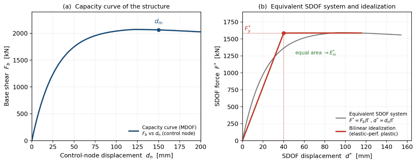
The capacity curve describes the actual structure, with many degrees of freedom (MDOF). The earthquake, however, is usually described by a response spectrum for a single-degree-of-freedom oscillator. The N2 method builds the bridge between these two worlds, and this is exactly the bridge that ETABS automates.
The N2 Method, Step by Step (EN 1998-1, Annex B)
The EC8 target displacement is obtained using the N2 method, which combines pushover analysis of an MDOF model with response-spectrum analysis of an equivalent SDOF system in acceleration/displacement format. It is worth going through the five steps, because these are precisely the steps that ETABS performs internally.
Equivalent SDOF System
The mass of the equivalent system and the transformation factor are obtained from the floor masses mᵢ and the normalized deformation shape Φᵢ, with Φ = 1 at the control node:
m* = Σ mᵢ Φᵢ
Γ = m* / Σ (mᵢ Φᵢ²)
The quantities of the equivalent system are obtained simply by dividing the force and displacement from the MDOF curve by the factor Γ:
F* = Fb / Γ d* = dn / Γ
Bilinear Idealization
The SDOF curve is idealized as elastic-perfectly plastic (Figure 1b). The plateau Fy* corresponds to the yield force of the idealized system, and the yield displacement is determined by imposing equality of deformation energy Em* up to the formation of the plastic mechanism (dm*):
dy* = 2 · ( dm* − Em* / Fy* )
Period of the Equivalent System
Using the mass and elastic stiffness of the idealized branch, the natural period of the equivalent SDOF system is:
T* = 2π · √( m* · dy* / Fy* )
Target Displacement of the Equivalent System
For the elastic system with period T*, the target displacement is that of the corresponding elastic oscillator, read directly from the elastic response spectrum Se:
det* = Se(T*) · [ T* / (2π) ]²
Short-Period Correction
The equal-displacement rule is only valid in the medium- and long-period range. If T* ≥ TC, dt* = det* is accepted. For short periods (T* < TC), the inelastic response is amplified:
dt* = ( det* / qu ) · [ 1 + ( qu − 1 ) · TC / T* ] ≥ det*
where qu is the ratio between the elastic acceleration and the yield acceleration of the equivalent system:
qu = Se(T*) · m* / Fy*
Return to the Real System
Finally, the target displacement of the real structure, at the control node, is recovered by multiplying by the same transformation factor:
dt = Γ · dt*
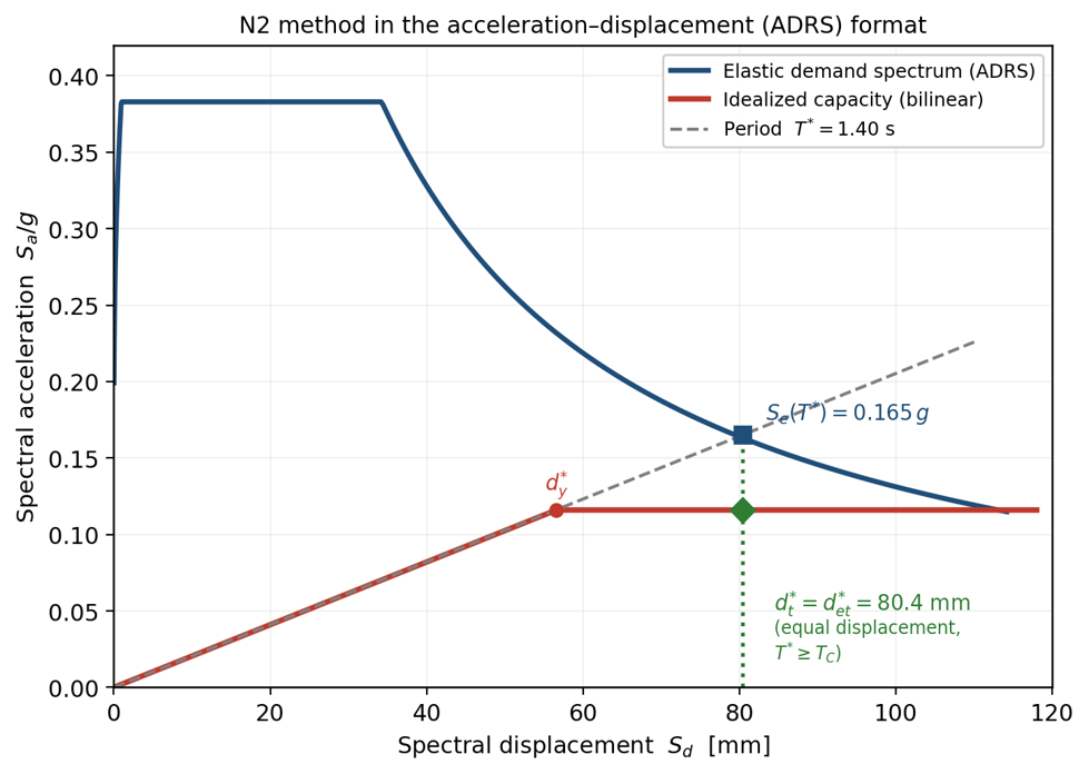
How ETABS Automates the N2 Method
The remarkable point is that this entire procedure is built into ETABS. The engineer defines the elastic spectrum, selects the pushover case, and ETABS returns the ADRS graph with the bilinear idealization, period T*, target displacement, and intermediate factors already included. The workflow, as applied in this model, is as follows.
Define the Elastic Response Spectrum
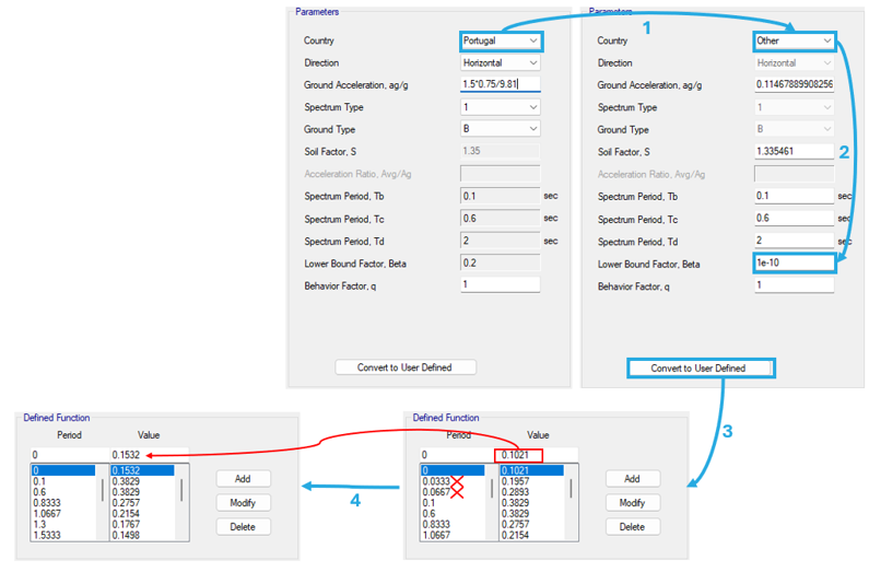
Under Define ▸ Functions ▸ Response Spectrum, the Eurocode 8, 2004 function is selected and the seismic action parameters are entered. In the case study, this corresponds to Type 1 seismic action, Zone 1.3, ground type B, and a 308-year return period. The sequence shown below allows the ETABS design spectrum to be transformed into an elastic spectrum.
The Result: the Building Target Displacement
This graph, EC 8 2004 Target Displacement, is the culmination of the entire process. It reflects all nonlinear characteristics assigned to the model, the resulting capacity curve, and the elastic spectrum AST1. It corresponds to the push_modal_X case (modal distribution, X direction) and provides the direct reading of the structure target displacement.
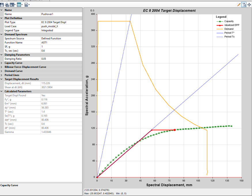
In the acceleration/displacement graph, the capacity curve is shown in green, the bilinear idealization in red, the reference seismic action spectrum in orange, and the period lines T* and TC in blue. ETABS solves the N2 method and reports, in the left-hand panel, all intermediate parameters and the final result.
| Parameter | Symbol | Value (ETABS) | Source |
|---|---|---|---|
| Transformation factor | Γ | 1,433 | MDOF↔SDOF transformation |
| Yield acceleration | Fy*/m* | 0,116 g | idealized SDOF plateau |
| Yield displacement | dy* | 56,585 mm | bilinear idealization |
| Equivalent period | T* | 1,40 s | 2π√(m*·dy*/Fy*) |
| Spectral acceleration at T* | Se(T*) | 0,165 g | read from the AST1 spectrum |
| Corner period | TC | 0,60 s | AST1 spectrum |
| Elastic target (SDOF) | det* | 80,406 mm | Se(T*)·(T*/2π)² |
| SDOF target (T* ≥ TC) | dt* | 80,406 mm | = det* (equal displacement) |
| Target displacement (control node) | dt | 115,226 mm | Γ · dt* |
| Base shear at target | V(dt) | 3021,6 kN | MDOF model response |
The complete calculation sequence, from the MDOF→SDOF transformation to the spectrum reading, is presented in Annex A, allowing each of these values to be reproduced independently.
The 150% Target Displacement Check
One practical point that ETABS helps control is that the capacity curve should extend to at least 150% of the target displacement. This requirement is not intended to check performance at the target point, but to encourage the engineer to investigate the behavior of the model under extreme loading conditions that exceed the values associated with the seismic risk level under consideration. It is the difference between knowing where the target is and knowing how much margin exists beyond it; in other words, whether the hinges still respond stably or whether load drops and undesirable mechanisms appear.
In Figure 3, this requirement can be read directly: the capacity curve, shown in green, extends beyond 1.5 × dt* ≈ 121 mm in spectral format, equivalent to approximately 173 mm at the control node. This is why the pushover cases were defined with a generous initial monitored displacement of 200 mm: it ensures that the analysis comfortably exceeds 150% of the target without having to rerun it.
Limitations and the Effect of Higher Modes
The basic form of the N2 method assumes a response dominated by the fundamental mode in each direction. This is an acceptable assumption for regular buildings, but it loses validity when higher modes become significant, either over the height of the structure or in plan through torsion. These are precisely the typical situations found in old, asymmetric buildings with irregular stiffness distributions.
The extended N2 method keeps the pushover analysis of a 3D model as its basis; this is what controls the target displacement and the distribution of nonlinear deformations over the height. It then corrects it using the results of an elastic modal response-spectrum analysis through two sets of factors:
-
Over the height, by comparing the normalized interstory drifts obtained from the modal analysis and from the pushover analysis, in order to recover the amplification in the upper stories that the pushover force distribution underestimates.
-
In plan, by comparing the normalized displacements in the same two analyses, in order to capture torsional amplification.
In both cases, the corrective factor is the ratio between the modal-analysis value and the pushover-analysis value, with a lower bound of 1.0: no reduction of demand is allowed, either over the height or on the stiff side. Accidental mass eccentricity should also be considered.
Attachments
 Anex A.pdf