
“Stress Averaging” in Shell Elements: Concept and Practical Example
In finite element models, especially when analyzing shells (slabs, walls, retaining walls, etc.), users often find it surprising that the values reported at a specific location depend on the elements present in the view or the chosen stress averaging option. This behavior is not always due to a modeling problem: it often results from how the software performs the averaging of stresses or forces. This article explains what this process entails and presents a simple example to illustrate why values can change depending on visible elements or the type of averaging used.
What is Stress Averaging?
Stress averaging is the process of smoothing (or averaging) stress or force values between elements that share the same joint. This process is present in all CSI finite element modeling programs (SAP2000, ETABS, SAFE, CSiBridge, etc.). In a finite element model, the forces of each element are calculated at their integration points (interior points), and, when presented at the joints, significant differences can arise from one element to another. To make the results appear more “smooth” or “uniform,” the program can average these values at the joint or simply keep them separate.
Why do values change when you change the visible elements?
The program defaults to stress averaging “At All Joints.” When performing this averaging at all joints, the software only considers the elements that are visible. Thus, when the user hides parts of the model (e.g., remove certain slabs or walls from view), those elements are excluded from the averaging. Consequently, different force values will be shown at the same joint.
Managing Stress Averaging
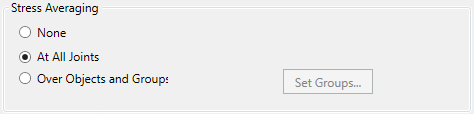
There are three main modes for displaying stresses and forces:
- None: no averaging of stresses or forces between elements sharing the same joint. Each element reports its own value at the same point.
- At All Joints: the program averages all the values of the elements sharing the joint and present in the view. This provides a more uniform global contour but can mask important discontinuities.
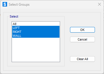
- Over Objects & Groups: averaging is only done within each selected object or group, without mixing forces from structurally distinct regions.
Practical Example
Consider a SAP2000 model with a small wall supported on a slab. We will analyze the results for a load case applying a lateral load at the top of the wall; the following image shows the deformed shape:
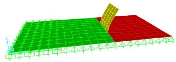
The different colors indicate the following three groups of objects:
- Green – group LEFT
- Yellow – group WALL
- Red – group RIGHT
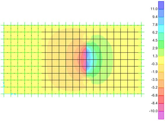
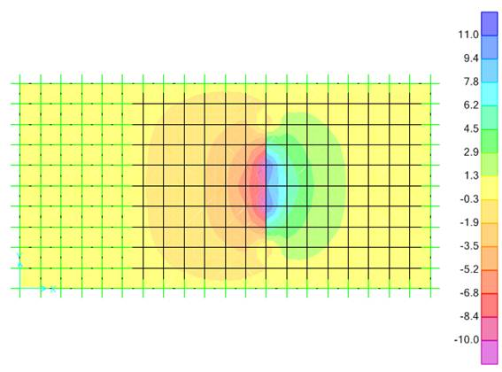
Moment M11 contours with “At All Joints” option (2D plan view):
.png)
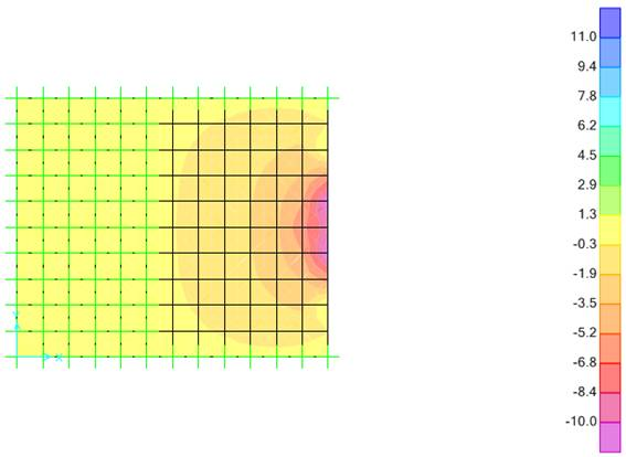
Moment M11 contours with “None” option (2D plan view):
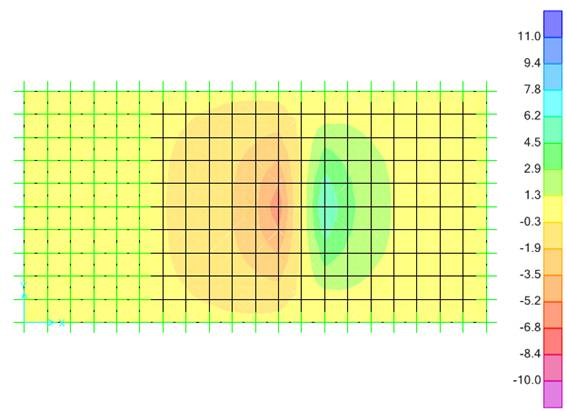
Moment M11 contours with “Groups” option (2D plan view):
Finally, if we exclude the objects on the right from the 2D view, the averaging is done solely among the objects on the left, even when using the default option (At All Joints):
The model can be downloaded from this article to easily replicate this behavior in SAP2000.
Advantages and precautions in use
- Detecting Critical Regions: using “None” helps identify stress concentrations. If there are very large discrepancies between adjacent elements, it may indicate that the mesh is not refined enough or that the local geometry requires more attention.
- Smoothing for Presentation: choosing “At All Joints” is useful in global reports since it gives a more unified view and facilitates the identification of maximum stress areas without excessive visual noise.
- Avoiding Improper Averages: in cases of discontinuity (e.g., the transition between a slab and a drop that absorbs more moments for the same curvature), choose “Over Objects & Groups” to calculate averages separately; thus, avoiding masking real force jumps.
Best practices
- Presentation Consistency: when comparing reports or screenshots, ensure you are using the same averaging option and the same set of visible elements.
- Local Verification: if you want to analyze exact stresses in a critical region, it is better to opt for “None”, avoiding averaging that may hide potential stress peaks.
- Global Assessment: if the primary interest is the overall behavior, “At All Joints” provides a more uniform contour.
- Discontinuities: where there are plane junctions that should not share forces, it is recommended to use “Over Objects & Groups” to avoid mixing regions with different behaviors.
Conclusion
Stress averaging in finite element programs greatly enhances the interpretation of results but directly depends on which elements are included in the averaging. The practical example above shows how hiding certain objects can change how the program presents the forces. Understanding how stress averaging works is essential to ensure report consistency and correctly compare results across different stages of analysis.
Final Note: stress averaging applies not only to forces or stresses but also to any other values reported for shell elements, such as the results obtained by the Concrete Shell Design in SAP2000 and CSiBridge.