Combining linear and nonlinear cases: what combinations can (and cannot) do.
The question arises in almost every model: can I add these cases together in a combination, or do I have to combine the loads within the Load Case itself? The answer depends on a central idea: superposition, and knowing when it ceases to be valid. In CSI programs, the way loads are organized determines whether results can be added after the analysis or if they must be combined beforehand. Confusing these two paths leads to results that appear correct but are physically wrong. The following sections clarify this boundary with two practical cases and the precautions to take when using envelopes in design.
Three levels that should not be confused
Before combining anything, it is useful to keep in mind the hierarchy shared by CSI programs. These are three distinct concepts, and most errors stem from treating them as if they were equivalent.
The first level is the Load Pattern: the spatial distribution of an action, such as DEAD, LIVE, WIND, or QUAKE. By itself, it does not produce any results; it is merely the definition of the load.
The second level is the Load Case, which defines how each pattern is applied and how the structure responds: statically or dynamically, linearly or nonlinearly, and in what sequence. This is where results are produced.
The third level is the Load Combination, which adds or envelopes the results of multiple Load Cases or other combinations. It operates on already calculated results.
The critical point lies in the jump from the second level to the third. A combination works on results that already exist, and it only makes sense to add results when those results are, in fact, superimposable.
The principle of superposition
In linear cases, superposition is valid. All linear cases rely on the same stiffness matrix, so their results can be superimposed: the effect of the dead load plus the effect of the live load is equal to the effect of the dead load and live load applied together. A combination of the type 1.2·DL + 1.6·LL is, therefore, perfectly legitimate. This is the foundation of almost all routine design: linear cases are defined at service levels, and the results are factored and combined at the combination level.
In nonlinear cases, superposition is no longer valid. Stiffness changes throughout the loading process, and the response depends on the order in which the loads are applied. The result of DL added to the result of LL is no longer equal to the result of DL + LL applied within the same analysis. The rule is clear: results from nonlinear analyses should not be superimposed. Instead, all loads acting together must be combined within the nonlinear Load Case itself, and these cases can be chained to represent loading sequences.
In summary, except for the Envelope type, combinations should generally apply only to linear cases, because nonlinear results are, as a rule, not superimposable.
The five types of linear combination
When working with linear results, the chosen combination type alters the meaning of the result. Five main types are available:
The Linear Add type multiplies each case by its respective scale factor and sums the results. It is the natural type for gravity and static loads and for code-prescribed combinations of linear cases, such as 1.2·DL + 1.6·LL.
The Absolute Add type sums the absolute values of the cases, automatically generating positive and negative values in each section. It is conservative because it assumes that the maximums coincide, and it is used for lateral loads when a safe-side estimate is intended.
The SRSS type computes the square root of the sum of the squares of the results, considering both positive and negative values. It is appropriate for combining contributions that do not necessarily occur in phase, such as seismic directions, modal results, or directional components.
The Envelope type evaluates the maximum and minimum in each section, storing two values per point. The case that gives rise to the maximum may be different from the one that gives rise to the minimum. It is the only type that can include nonlinear cases and is used for moving loads or any situation where obtaining extreme values is important. Note: it does not represent a single state of equilibrium, as detailed in the section on envelope precautions in design.
The Range Add type defines the combined maximum as the sum of the positive maximums of each contributing case, and the combined minimum as the sum of the negative minimums. It resolves with a single combination what would otherwise require hundreds of checkerboard load permutations, making it ideal for alternating live loads on floors and bridge decks.
Practical case: a nonlinear combination
The goal is to obtain the combination 1.2·DL + 1.6·LL in a frame where P-Delta effects are relevant. The temptation is to run DL and LL as separate nonlinear cases and add them in a combination. This procedure is wrong because nonlinear results do not superimpose. The most rigorous way, respecting the loading sequence and the nonlinearity of the factored loads, is as follows:
- Create a nonlinear Load Case DL where the DL pattern is applied already with the 1.2 factor.
- Create a nonlinear Load Case LL where the LL pattern is applied with the 1.6 factor.
- Indicate that the LL case continues from the stiffness at the end of the DL case (continue from state at end of nonlinear case). The live load enters onto the structure already deformed by the dead load.
- Perform the design based on the LL case, which incorporates the accumulated effect of the sequence.
If the sequence is not important but the nonlinearity is, simply create a single nonlinear case with DL at 1.2 and LL at 1.6 applied together. When nonlinearity is minor, the classical method of linear cases at service levels, added in a combination, remains reasonable.
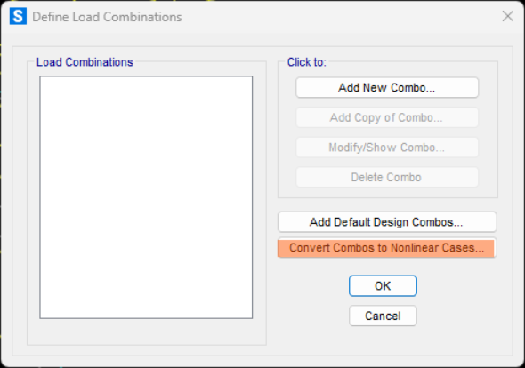
The shortcut Convert Combinations to Nonlinear Cases automates the conversion, generating P-Delta nonlinear cases.
A practical note for buildings: for P-Delta, the standard procedure is to define a single initial P-Delta case under gravity load and then run the remaining analyses (static, modal, spectrum, or Time History) linearly over that stiffness. Only when the interaction of axial force with a specific lateral combination is critical is a dedicated nonlinear P-Delta case justified for that combination. If you want to know more about this topic, see our course Geometric Nonlinearity.
Practical case: a linear combination
The response spectrum is a linear case, but it loses sign and phase: a maximum is calculated for each mode, and these maximums do not necessarily occur simultaneously. The combination is done in stages before reaching the final combination:
- Combine (via Load Case) the modal contributions using CQC, which accounts for damping and equates to SRSS when damping is zero, or directly with SRSS.
- Combine (via Load Case) the directions, for example SPECX and SPECY, by SRSS or the 100/30 rule.
- Add the seismic result to the gravity load in a Linear Add type combination.
- Let the program generate the sign and interaction permutations in the design phase, rather than constructing them by hand.
Since response spectrum results are always positive, the program associates the extreme values with the static case in all possible sign combinations. This is what guarantees a correct verification of the P-M-M interaction, which might otherwise be lost.
Precautions with envelopes in design
Do not assign an Envelope type combination as a design combination. An envelope stores the maximum and minimum per section, and these extremes can come from different cases. It does not represent a single state of equilibrium or a set of concurrent forces. Designing a column for the maximum axial force from one case and the maximum moment from another, when they never occur at the same time, breaks the necessary correspondence for P-M-M interaction and leads to an unrealistic design.
CSI programs treat each combination separately, generate the design for each one, and only then envelope the set of results. An envelope defined manually over design combinations can generate capacity for an extreme loading that, in practice, does not exist. The image below shows how to correctly define design combinations.
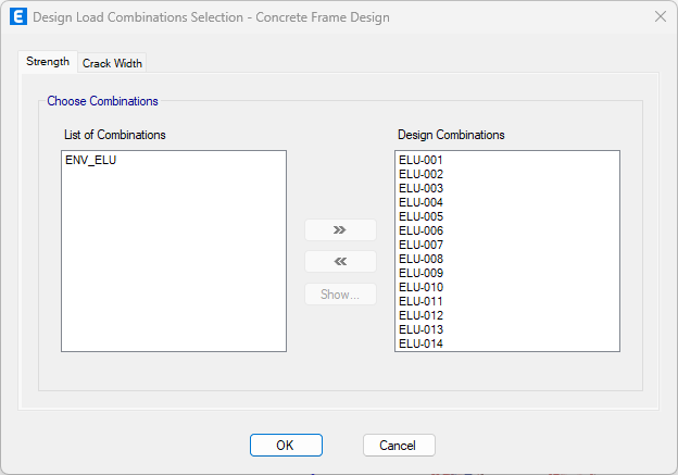
The recommendation is clear: do not envelope design combinations. All combinations should be added individually, letting the software design and report the results for each section, identifying the governing case.
Practical case: Time History Load Case
If the Time History analysis is linear, its results can be combined with other linear cases through Load Combinations, provided that the chosen combination type correctly represents the phenomenon in question. Still, it is worth remembering that a Time History already contains a full history of response, not just an isolated static value.
If the Time History analysis is nonlinear, the logic changes: the results should not be added later in an additive combination.
A typical example is a structure that first receives gravity loads and only then is subjected to a seismic action over time. In this case, an initial nonlinear gravity case must be created first, with dead loads and other necessary actions, followed by a Time History case that continues from the final state of that initial case. Thus, the dynamic excitation acts on the already deformed structure with the stiffness corresponding to the gravity state.
Envelopes can be useful for checking maximums and minimums over time, or for comparing multiple time histories, but they should not be confused with a design combination. Just like with other envelopes, the maximum axial force value and the maximum moment value can occur at different times, or even in different time histories. The envelope is a tool for reading extremes, not a unique state of equilibrium.
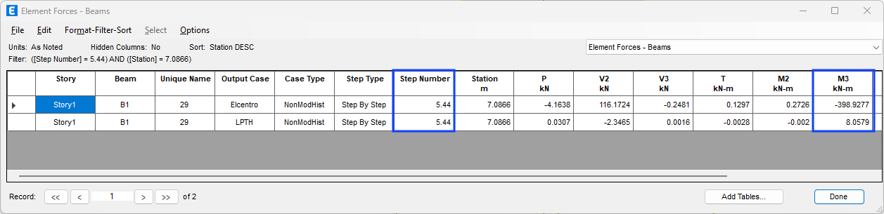
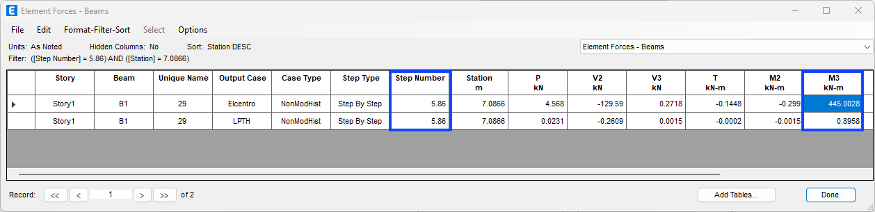
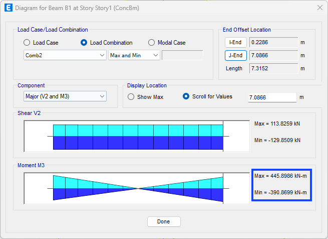
The difference between how a Linear Add combination of Time History cases is treated in design versus result analysis is presented below.
Design
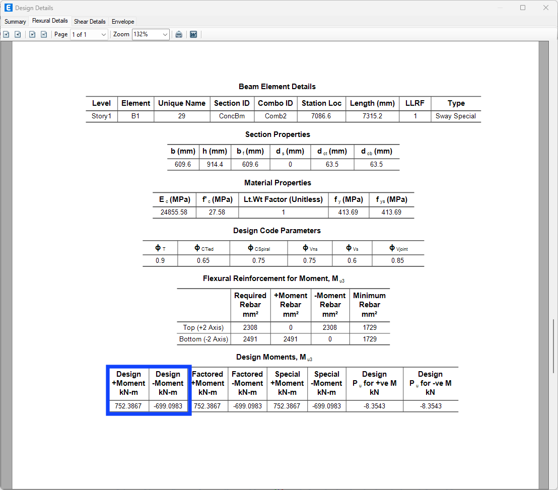
For design, the software first identifies the maximum and minimum moments in each Time History. It then applies the combination factors and sums the maximums together and the minimums together. In the example, a Linear Add combination of 2 Time History type Load Cases was performed for design purposes.
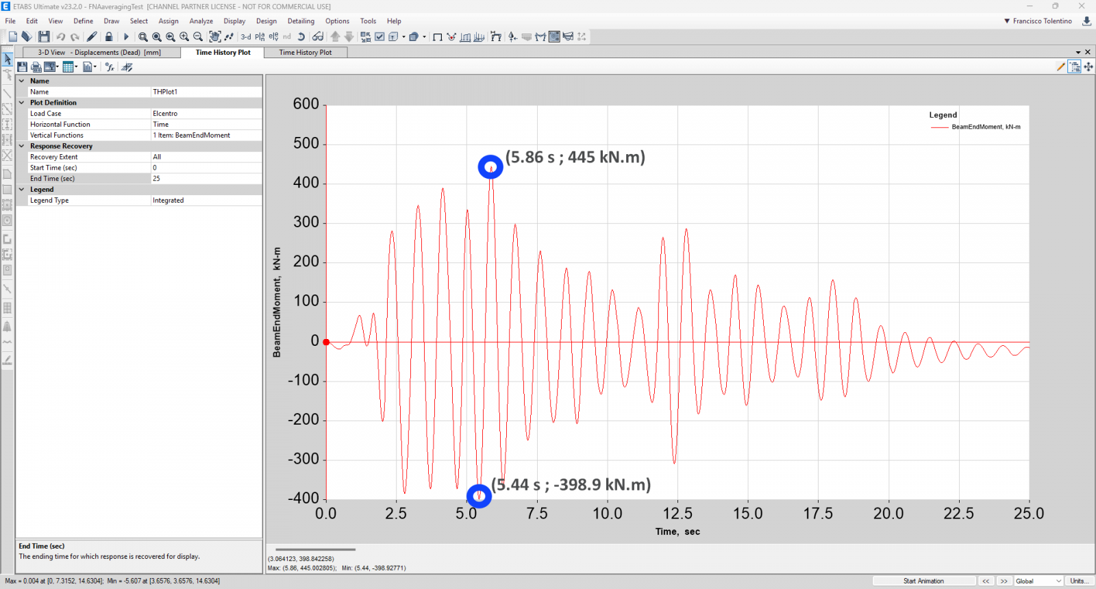
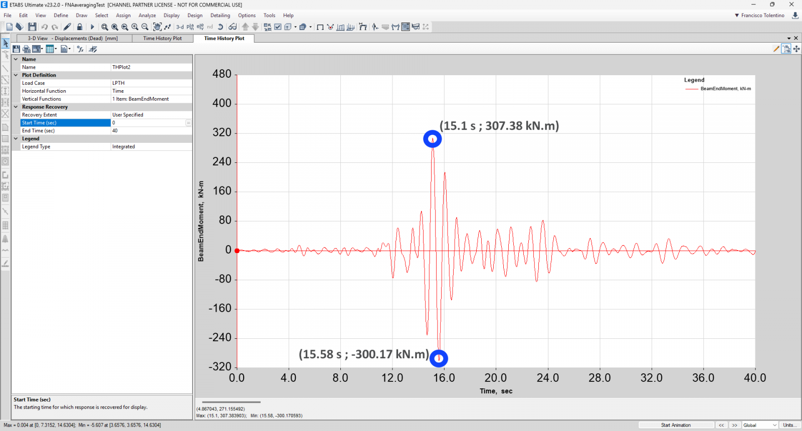
The maximum of this combination results from 445 + 307 = 752 kN.m. The minimum results from -398.92 + (-300.17) = -699 kN.m. These values represent an envelope for design, not a response at a single instant of the analysis, as can be observed and verified through the step value, which in this case corresponds to the time stamp of the record.
Analysis of results
In result analysis, the logic is different. The program sums the forces of the various Time History cases at the exact same step and only then looks for the extremes of the combination. In the example, the maximum occurs at time 5.44 s: -398.92 + 8.06 = -390.86 kN.m. The minimum occurs at time 5.86 s: 445.00 + 0.90 = 445.90 kN.m. The analysis values are lower than the design values because they respect the temporal simultaneity of the results.