Solution Control for Nonlinear Analysis in CSI Software 

When you venture into the world of nonlinear analysis in programs like SAP2000, ETABS, and CSiBridge, you're asking the software to solve a much more complex puzzle than a standard linear analysis. The structure's behavior changes as loads are applied. The "Nonlinear Parameters (Solution Control)" dialog box is your command center for guiding the software on how to solve this puzzle, especially when the analysis is demanding and struggles to find a solution (converge). 

This guide simplifies these advanced settings to help you optimize your calculations and achieve convergence. 

How to Access Solution Control 

1. Go to the Define menu and select Load Cases. 
2. Create a new load case or modify an existing one. 
3. In the Load Case Data form, set the Analysis Type to Nonlinear or Nonlinear Staged Construction. For time-history analysis, choose Nonlinear as the type and Direct Integration or Modal as the subtype. 
4. Click the Nonlinear Parameters button to open the Solution Control settings. 

The Core Concept: Solution Schemes 

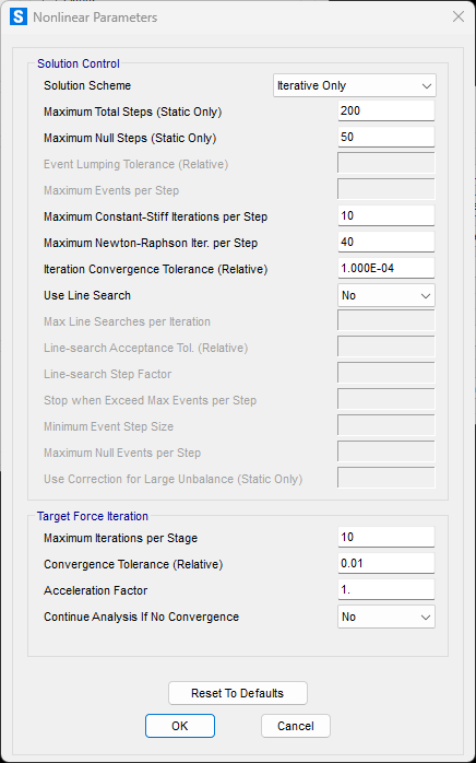
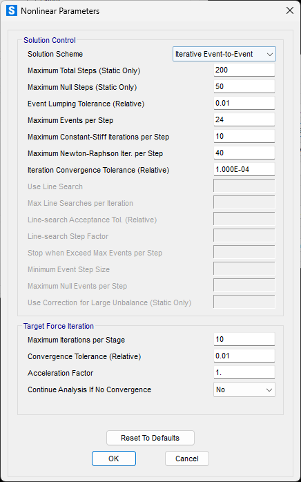
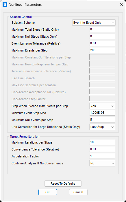
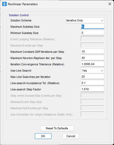
The most critical choice you'll make is the Solution Scheme. This determines the fundamental strategy the solver uses. The options vary slightly depending on whether you're running a static or time-history analysis. 

• Iterative Only: This is the most straightforward approach. The solver applies a portion of the load and then iterates—repeating calculations—until the forces in the structure are balanced (in equilibrium). It prioritizes accuracy by ensuring equilibrium is met at the end of each step.

• Iterative Event-to-Event: This is a hybrid approach. It uses the efficient Event-to-Event stepping to subdivide the load steps where stiffness changes significantly, but it also performs iterations at the end of each step to ensure equilibrium is achieved. This provides a balance between the speed of event stepping and the accuracy of iteration. 

• Event-to-Event Only: This scheme focuses on speed and overcoming convergence difficulties. The solver doesn't iterate to check for equilibrium. Instead, it precisely calculates the load required to cause the next "event" (like a hinge yielding or a cable going slack) and steps directly to that point.
  • Advantage:  It's fast and can often complete an analysis that otherwise fails. 
  • Caution: Because equilibrium is not explicitly checked at each step, you must carefully review the results to ensure the equilibrium error is acceptably small.

Key Parameters for All Nonlinear Analyses 

While some parameters are specific to the analysis type, a few general ones are important to understand. 

• Maximum Total Steps: This is a safety control that limits the total number of steps (both saved and intermediate) the analysis will perform. If your analysis stops before reaching the target load, it's often because it hits this limit. Solution: Rerun the analysis with a higher value. Start with a smaller number to gauge the analysis time. 
• Maximum Null Steps: Null steps are "zero-progress" steps that occur when the solver is struggling, such as when a hinge unloads or iterations fail to converge. An excessive number of null steps indicates the solution might be stalled due to instability or numerical sensitivity. This parameter allows you to terminate a failing analysis early instead of letting it run indefinitely. To disable this check, you can set it equal to the Maximum Total Steps. 

Parameters for Nonlinear Static & Staged-Construction Analysis 

Besides the Solution Scheme, a key option is: 

• Use Line Search: When set to 'Yes' for iterative schemes, this algorithm helps find a better solution more efficiently during iterations. It scales the solution increment in a trial-and-error way to reduce the force unbalance. This can lead to better convergence with fewer overall iterations, even though each iteration takes slightly longer. Note that it is not used for Event-to-Event schemes. 

Parâmetros para Análise Dinâmica Não-Linear por Integração Direta (Nonlinear Direct-Integration Time-History) 

The accuracy of direct-integration methods is very sensitive to integration time step, especially for stiff (high-frequency) response. Try decreasing the maximum substep size until consistent results are obtained. Keep the output time step size fixed to prevent storing excessive amounts of data. 

The analysis will always stop at every output time step, and at every time step where one of the input time-history functions is defined. In addition, an upper limit on the step size used for integration may be set. For example, suppose the output time step size was 0.005, and the input functions were also defined at 0.005 second. If the Maximum Substep Size is set to 0.001, the program will internally take five integration substeps for every saved output time step. The program may use smaller substeps if necessary to achieve convergence when iterating. 

Note: The default value of zero means no limit, i.e., use the output time-step size. 

Parameters for Nonlinear Modal Time-History (FNA) 

Modal analysis is generally less sensitive to step size than direct integration. The main reason for limiting the maximum substep size is for comparison with other analyses that have used such limits. 

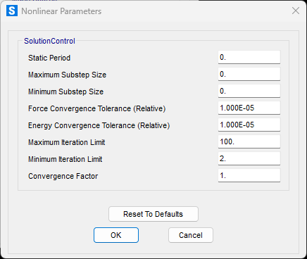
• Static Period: Normally all modes are treated as being dynamic. Optionally this parameter may be used to specify that high-frequency (short period) modes be treated as static, so that they follow the load without any transient response. This may be useful for certain quasi-static analyses. Usually, however, the iteration is more stable if dynamic effects are included. 

• Force and Energy Convergence Tolerance: These values define "how close is close enough" for the solver. The Force Tolerance compares the force error to the total forces on the structure. The Energy Tolerance is a secondary check to limit the amount of nonlinearity allowed within a single substep. 

• Iteration Limits (Max/Min): These control the number of iterations allowed for each substep. The program automatically balances between allowing more iterations and reducing the step size. The default values typically work well. 

• Convergence Factor: Under-relaxation of the force iteration may be used by setting the convergence factor to a value much less than unity (i.e., 0.1 to 0.01). Smaller values increase the stability of the iteration, but require more iterations to achieve convergence. 

Understanding Target-Force Iteration 

Target-Force Iteration is a special process that balances forces in your model before the main analysis step begins. It is most useful when a structure starts in a highly unbalanced state. 

How It Works 

When you apply loads with a "target force" in a nonlinear static analysis, the software uses an iterative process to reach those targets. 

1. Initial Analysis: The software applies trial loads to the elements you assigned a target force to and runs a complete nonlinear analysis (or a single stage of it). 

2. Compare and Calculate Error: After the analysis, it compares the actual forces in those elements to your target forces. It then calculates an average error. 

3. Repeat: If the error is larger than the convergence tolerance you set, the software calculates a new trial load and runs the entire analysis again. 

This process repeats until the error is within the tolerance or the maximum number of iterations is reached. 

Control Parameters 

You can control this process using the following settings in the nonlinear static Load Case: 

• Relative Convergence Tolerance: This defines the acceptable error level for the target forces. Since these are desired targets and not required for equilibrium, a larger value like 0.01 to 0.10 is often recommended.
• Maximum Number of Iterations: This sets a limit on how many times the process can run. It's a good idea to start with a moderate value, like 5 to 10, and increase it if needed.
• Acceleration Factor: This factor adjusts the load for the next iteration.

  • Use a value greater than 1 if convergence is slow (e.g., when pushing against a flexible structure). 

  • Use a value less than 1 if the process is unstable and the error is growing or fluctuating. 

• Continue on Failure: You can choose to continue the main analysis even if the target forces are not perfectly met. This is useful because achieving the exact target may not always be possible or necessary.

Tips and Best Practices 

• Be Realistic: You cannot force arbitrary loads onto a simple, statically determinate structure (like a basic truss). The process works best on stiff, complex structures with multiple supports. 

• Expect Slow Convergence: Convergence can be slow when target elements are connected to very flexible supports or work against other target-force elements. 

• Separate Load Cases: For better results, try to apply target-force loads in a separate Load Case or construction stage from other types of loads whenever possible.