SAP2000 and CSIBridge Cable Element and Shape Finder 

What is a cable element? 

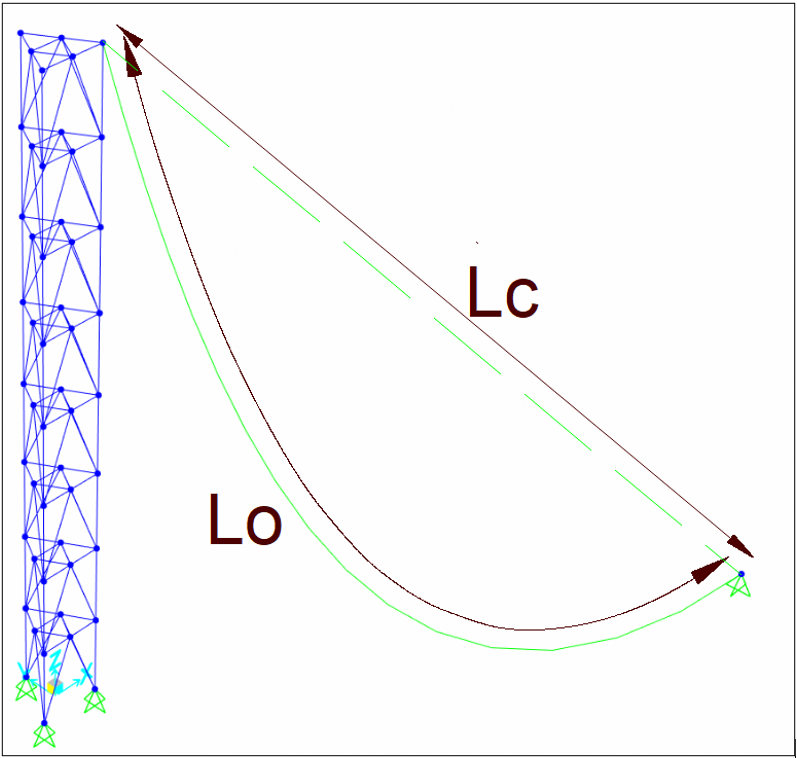
The Cable element models the catenary behavior of a slender, tensiononly member. It has axial stiffness but no bending or shear stiffness, and its response includes largedeflection and tensionstiffening effects, so analysis is nonlinear by nature. A cable connects two joints (I and J); mass for dynamics is by default lumped at these joints. Behavior is governed mainly by the undeformed length L₀ compared with the endtoend chord Lc: if L₀ ≈ Lc the cable is just taut; if L₀ > Lc it sags. 

When to use it 

Choose the Cable element when axial force dominates and sag under gravity is relevant. Typical applications include suspension and stay cables, hangers for girders or roofs, tension ties and bracing, guyed masts, and façade or canopy cables. Use frame elements instead if you must capture bending/shear behavior or complex material nonlinearity along the member. 

How the software calculates the cable shape  

The Cable Layout (shapefinding) tool solves for L₀ so the cable satisfies a condition you choose—such as a target end tension, a specified sag, or a horizontal tension component—under preview loads. These preview loads (selfweight, optional added weight per unit length, and optional projected uniform gravity load) exist only to determine the starting geometry; they are not analysis loads.  

The computed geometry is an initial state; actual results will depend on the full model, support movements, and the loads you apply in load cases. If no transverse load exists and the cable is slack, a small weight is assumed to obtain a unique shape, but best practice is to stabilize with realistic gravity or distributed load. 

Shape Finder Form options 

The Cable Type menu defines the condition used during shapefinding: 

• Undeformed Length (you enter L₀) or Relative Undeformed Length (you enter L₀/Lc) when geometry is known. 
• Tension at IEnd or JEnd, or Horizontal Tension Component, when you want to tune forces. 
• Minimum Tension at IEnd or JEnd to find the L₀ that minimizes the selected end force. 
• Maximum Vertical Sag or LowPoint Vertical Sag to target geometry rather than force. 

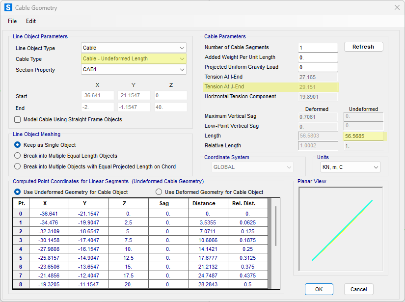
The form reports end tensions, horizontal component, sag values, L₀ and L₀/Lc, and displays computed point coordinates. “Added Weight per Unit Length” and “Projected Uniform Gravity Load” affect only the layout calculation. Set the “Number of Cable Segments” for meshing; one segment is usually adequate for catenary behavior, while multiple segments are helpful for pointload application or vibration studies. 

Loads used in analysis 

During analysis, you can activate selfweight (downward along arc length), apply Gravity Load with a chosen direction and scale, and use Distributed Span Load (uniform or trapezoidal referenced to undeformed length). Temperature loads add thermal strain; axial strain/deformation loads lengthen or shorten the cable directly; TargetForce loads iteratively impose a final desired tension at a specified relative location in a nonlinear static or staged case. Point loads should be applied at joints, so split the cable where the load acts. 

Analysis requirements and solver tips 

The correct analytical approach involves a two-stage process: 

1. Initial Nonlinear Static Case: The primary objective is to find the initial equilibrium state of the cables under a stabilizing load, typically self-weight. This is achieved by defining a Nonlinear Static or Staged Construction load case. During this analysis, the solver employs an iterative procedure, such as the Newton-Raphson method, to solve the nonlinear equilibrium equations. It repeatedly updates the tangent stiffness matrix and calculates the unbalanced load vector (the residual between internal forces and external loads) until it converges within a specified tolerance. 
    
2. Stiffness for Subsequent Analyses: Once this initial case has converged, the structure has a realistic, physically stable configuration where cables are properly tensioned. Any subsequent analysis, such as a linear static case for service loads or a Modal analysis for determining natural frequencies, must be defined to "Use Stiffness at End of Nonlinear Case." This instructs the software to build its initial stiffness matrix from the final, tensioned state of the preceding nonlinear analysis, ensuring accurate results. 

Achieving convergence in a nonlinear analysis can be challenging. For models utilizing the dedicated catenary cable element, the following solver adjustments within the nonlinear load case settings can significantly improve performance: 

• Fewer Segments: The catenary element's formulation mathematically describes the entire curve between its nodes. Therefore, a single element is typically sufficient and numerically efficient. Discretizing a cable into multiple catenary segments is generally unnecessary and can sometimes complicate the solution path for the solver. 
• Larger Load Increments: Unlike frame element approximations of cables which require many small steps, the catenary element's robust formulation often allows the solver to find its final equilibrium position more directly. Using fewer, larger load application steps can be more effective and stable. 
• Increased Maximum Iterations: The solver performs a series of iterations within each load step to reduce the unbalanced load to zero. The Maximum Iterations Per Step parameter dictates how many attempts the solver is allowed before it reports a non-convergence error. Increasing this value from its default provides the Newton-Raphson algorithm with more opportunities to find a convergent solution, which is often necessary for geometrically sensitive models. 

Staged Construction Considerations 

When modeling with staged construction, be aware that activating a taut cable (where undeformed length L₀ is less than the chord length Lc) will induce an immediate tensile force. This action creates an initial unbalanced load vector at the beginning of that stage, requiring the solver to perform iterations to establish equilibrium before applying any other external loads defined for that stage. 

Cautions and good practice 

• Do not mistake shapefinding inputs for real loads; always define loads in Load Patterns and Load Cases. 
• Verify L₀ and L₀/Lc because small changes around Lc can switch the cable from slack to taut and dramatically alter tension. 
• Keep segmentation minimal unless you need joints for loads or detailed dynamics; unnecessary segments can slow convergence. 
• Mind local axes: distributed loads in local directions are referenced to the chord, not the sagged curve. 
• Remember that the cable carries only axial tension; use frames if bending or shear stiffness matters. 

A compact workflow 

1. Draw the cable between supports and open the Cable Layout tool. 
2. Choose a Cable Type (forcebased or sagbased) and include preview loads to compute a reasonable L₀. 
3. Set segments (often 1) and confirm the preview shape. 
4. Assign real loads: selfweight/gravity, distributed loads, temperature or strain/deformation, and any targetforce. 
5. Run a stabilizing nonlinear static or staged case, then review end forces, sag, and deflections; iterate L₀ or loads as needed. 

Practical example 

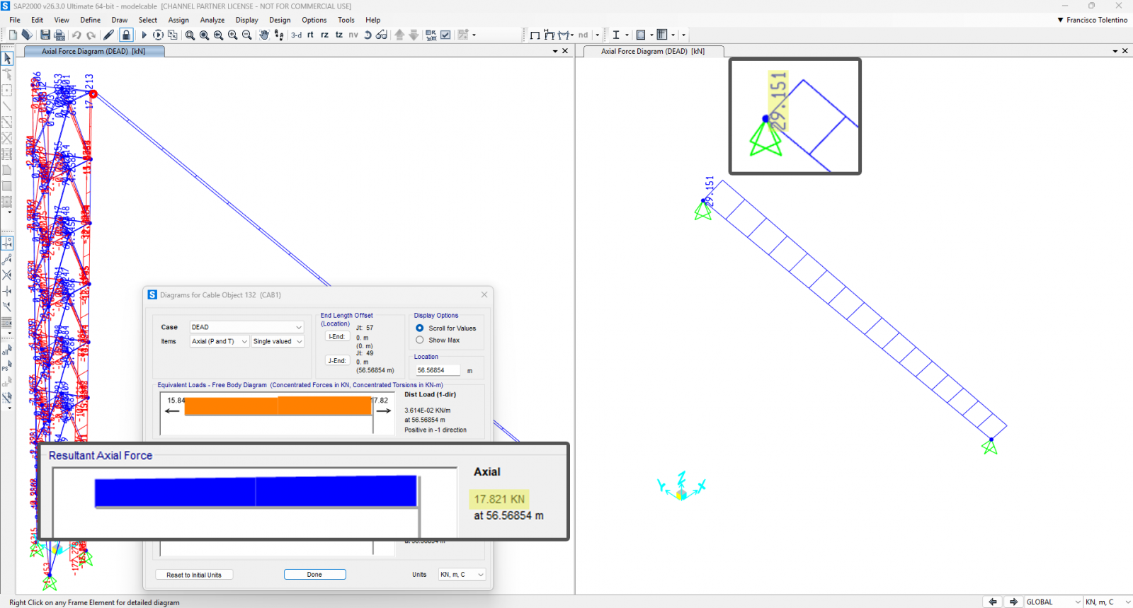
The following example shows how to implement a cable in a simple structure. The goal is to understand how the Shape Finder works. As a starting point, select the Undeformed Length criterion to make the cable nearly taut. 

With this setup, the target tension at the Jend is 29.151 kN. This value corresponds to the ideal case of fully restrained ends; once the cable is connected to a structure with some flexibility, the actual force will be lower. 

In the figure, the left model places the cable on a transmission tower, while the right model connects the cable between two restrained joints. 

As expected, the resulting axial force at the Jend in the tower model is lower than the value computed by the Shape Finder because the supports deform. In the restrainedjoints case, the axial force matches the Shape Finder result.